38 excel chart remove data labels
How to remove chart border in Excel? - ExtendOffice You just need to follow the below steps can remove the chart border. 1. Right click at the chart area and select Format Chart Area from the context menu. See screenshot: 2. In the Format Chart Area dialog, click Border Color in left pane, and then check No line option in the right section. See screenshot: 3. Excel Chart - Do not Hide Horizontal Data Label - Stack Overflow To answer your questions: Brief: 1) You can't see all your data labels on the X axis unless you format the X axis to have major interval of 1. 2) With a scatter plot, you cannot have your original labels retained on the X axis and, in your case, as your dates are recognised , they are ordered as such. You would need to convert the dates to text ...
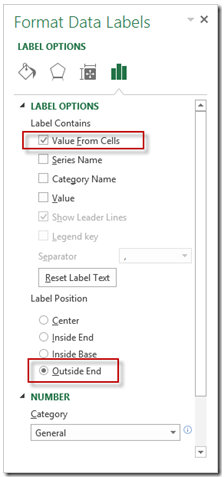
› charts › dynamic-chart-dataCreate Dynamic Chart Data Labels with Slicers - Excel Campus Feb 10, 2016 · Typically a chart will display data labels based on the underlying source data for the chart. In Excel 2013 a new feature called “Value from Cells” was introduced. This feature allows us to specify the a range that we want to use for the labels. Since our data labels will change between a currency ($) and percentage (%) formats, we need a ...

Excel chart remove data labels
Show or hide a chart legend or data table Select a chart and then select the plus sign to the top right. Point to Legend and select the arrow next to it. Choose where you want the legend to appear in your chart. Hide a chart legend Select a legend to hide. Press Delete. Show or hide a data table Select a chart and then select the plus sign to the top right. excel - Remove data label if less than a value - Stack Overflow You are removing the DataLabels for the entire series in this code. What you need to do is remove the DataLabel for the specific point on the series. This should do it: Dim cht As Chart Set cht = ActiveChart If Range ("B8") < 0.01 Then cht.SeriesCollection (1).Points (1).DataLabel.Delete End If. SeriesCollection (1) is the first series in the ... Enable or Disable Excel Data Labels at the click of a button - How To Select and to go Insert tab > Charts group > Click column charts button > click 2D column chart. This will insert a new chart in the worksheet. Step 2: Having chart selected go to design tab > click add chart element button > hover over data labels > click outside end or whatever you feel fit. This will enable the data labels for the chart.
Excel chart remove data labels. How can I hide 0-value data labels in an Excel Chart? How can I hide 0-value data labels in an Excel Chart? Right click on a label and select Format Data Labels. Go to Number and select Custom. Enter #"" as the custom number format. Repeat for the other series labels. Zeros will now format as blank. NOTE This answer is based on Excel 2010, but should work in all versions. How to Use Cell Values for Excel Chart Labels Select the chart, choose the "Chart Elements" option, click the "Data Labels" arrow, and then "More Options.". Uncheck the "Value" box and check the "Value From Cells" box. Select cells C2:C6 to use for the data label range and then click the "OK" button. The values from these cells are now used for the chart data labels. Prevent Overlapping Data Labels in Excel Charts - Peltier Tech Overlapping Data Labels. Data labels are terribly tedious to apply to slope charts, since these labels have to be positioned to the left of the first point and to the right of the last point of each series. This means the labels have to be tediously selected one by one, even to apply "standard" alignments. Excel Chart Data Labels - Microsoft Community Right-click a data point on your chart, from the context menu choose Format Data Labels ..., choose Label Options > Label Contains Value from Cells > Select Range. In the Data Label Range dialog box, verify that the range includes all 26 cells. When I paste your data into a worksheet, the XY Scatter data is in A2:B27, and the data labels are in ...
Excel chart labels keep coming back - Microsoft Tech Community Excel chart labels keep coming back I have a data set that I have changed the data labels for to reflect the total count of the objects in a functional category (vertical axes) with the bars of the chart broken up by the material type of the objects in the functional category. Adding/Removing Data Labels in Charts - Excel General - OzGrid #1 I need to know about the .HasDataLabels function After reading previous posts (particularly by norie and laplacian) I've decided that to remove a label from a single data point in a series on a chart I can't use the .HasDataLabels = false function, since it only applies to series objects. › documents › excelHow to rotate axis labels in chart in Excel? - ExtendOffice Rotate axis labels in Excel 2007/2010. 1. Right click at the axis you want to rotate its labels, select Format Axis from the context menu. See screenshot: 2. In the Format Axis dialog, click Alignment tab and go to the Text Layout section to select the direction you need from the list box of Text direction. See screenshot: 3. How to remove a legend label without removing the data series In Excel 2016 it is same, but you need to click twice. - Click the legend to select total legend - Then click on the specific legend which you want to remove. - And then press DELETE. If my reply answers your question then please mark as "Answer", it would help others to find their solution easily from your experience. Thanks Report abuse
excel - remove data labels automatically for new columns in pivot chart ... remove data labels automatically for new columns in pivot chart? I have a query that populates data set for a pivot table. I want data labels to always be at none. Whenever a new column shows up the data label comes back. Anyway I can permanently remove them from the entire pivot chart? Change the format of data labels in a chart To get there, after adding your data labels, select the data label to format, and then click Chart Elements > Data Labels > More Options. To go to the appropriate area, click one of the four icons ( Fill & Line, Effects, Size & Properties ( Layout & Properties in Outlook or Word), or Label Options) shown here. Add / Move Data Labels in Charts - Excel & Google Sheets Double Click Chart Select Customize under Chart Editor Select Series 4. Check Data Labels 5. Select which Position to move the data labels in comparison to the bars. Final Graph with Google Sheets After moving the dataset to the center, you can see the final graph has the data labels where we want. How to suppress 0 values in an Excel chart | TechRepublic Select the data set (in this case, it's B2:D9) Click Find & Select in the Editing group on the Home tab, and choose Replace. In Excel 2003, choose Replace from the Edit menu. In all versions, you...
Do My Excel Blog: How to hide the zero percent labels in an Excel pie chart
How to add data labels from different column in an Excel chart? Please do as follows: 1. Right click the data series in the chart, and select Add Data Labels > Add Data Labels from the context menu to add data labels. 2. Right click the data series, and select Format Data Labels from the context menu. 3.
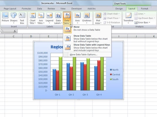
How to Add a Data Table to an Excel 2007 Chart - dummies
Excel Chart delete individual Data Labels First select a data label, which will select all data labels in the series. You should see dark dots selecting each data label. Now select the data label to be deleted. This should remove the selection from all other labels and leave the specific data label with white selection dots. Deletion now will remove just the selected data point.

Microsoft Excel Tutorials: The Chart Layout Panels
Edit titles or data labels in a chart - support.microsoft.com The first click selects the data labels for the whole data series, and the second click selects the individual data label. Right-click the data label, and then click Format Data Label or Format Data Labels. Click Label Options if it's not selected, and then select the Reset Label Text check box. Top of Page
How-to Use Data Labels from a Range in an Excel Chart - Excel Dashboard Templates
Remove zero data labels on chart - Excel Help Forum Over chart area, right button options, click Select Data. At dialog box, click Hidden and blank cells. At new dialog box, click Show data in hidden rows and columns. Not sure about precise English version for those commands, but they will show something like that. Godspeed! Last edited by Estevaoba; 07-25-2017 at 05:14 PM . Register To Reply

How to Add Data Labels to an Excel 2010 Chart - dummies
Add or remove data labels in a chart - support.microsoft.com On the Design tab, in the Chart Layouts group, click Add Chart Element, choose Data Labels, and then click None. Click a data label one time to select all data labels in a data series or two times to select just one data label that you want to delete, and then press DELETE. Right-click a data label, and then click Delete.
Add or remove data labels in a chart - Office Support
Move data labels - support.microsoft.com If you decide the labels make your chart look too cluttered, you can remove any or all of them by clicking the data labels and then pressing Delete. Tip: If the text inside the data labels is small, click and drag the data labels to the size you want. You can also change their format to make them easier to read. Need more help? Expand your skills

How to Add Data Labels to your Excel Chart in Excel 2013 - YouTube
How to add or move data labels in Excel chart? - ExtendOffice In Excel 2013 or 2016. 1. Click the chart to show the Chart Elements button . 2. Then click the Chart Elements, and check Data Labels, then you can click the arrow to choose an option about the data labels in the sub menu. See screenshot: In Excel 2010 or 2007. 1. click on the chart to show the Layout tab in the Chart Tools group. See ...
Excel Charts: Polar Plot Chart. Polar Plot Created Using Radar Chart
Format Data Labels in Excel- Instructions - TeachUcomp, Inc. To format data labels in Excel, choose the set of data labels to format. To do this, click the "Format" tab within the "Chart Tools" contextual tab in the Ribbon. Then select the data labels to format from the "Chart Elements" drop-down in the "Current Selection" button group. Then click the "Format Selection" button that ...
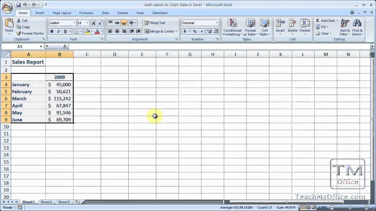
Add Labels to Chart Data in Excel - YouTube
How to Customize Your Excel Pivot Chart Data Labels - dummies To remove the labels, select the None command. If you want to specify what Excel should use for the data label, choose the More Data Labels Options command from the Data Labels menu. Excel displays the Format Data Labels pane. Check the box that corresponds to the bit of pivot table or Excel table information that you want to use as the label.

Microsoft Excel Tutorials: The Chart Layout Panels
How to add or remove data labels with a click - Goodly Change the data labels to match the color of the bar (it reads easier that way) The legends (for dummy calculations need to be removed) Click on the legend and then click again to only select dummy legend Press delete DOWNLOAD THE ADD REMOVE DATA LABEL CHART - Excel file The file also contains a cool VBA method that you can try it out..

How to get Excel Chart Columns with no gaps • AuditExcel.co.za
support.microsoft.com › en-us › officeSelect data for a chart - support.microsoft.com For this chart. Arrange the data. Column, bar, line, area, or radar chart. In columns or rows, like this: Pie chart. This chart uses one set of values (called a data series). In one column or row, and one column or row of labels, like this: Doughnut chart. This chart can use one or more data series

Elements of an Excel Chart | ExcelDemy.com
How to hide zero data labels in chart in Excel? - ExtendOffice Sometimes, you may add data labels in chart for making the data value more clearly and directly in Excel. But in some cases, there are zero data labels in the chart, and you may want to hide these zero data labels. Here I will tell you a quick way to hide the zero data labels in Excel at once. Hide zero data labels in chart
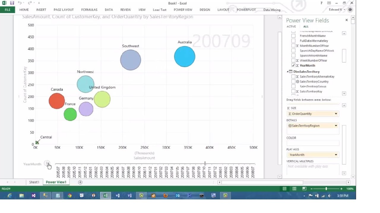
Excel 2013 PowerView Animated Scatterplot/Bubble Chart Business Intelligence Tutorial - YouTube
Enable or Disable Excel Data Labels at the click of a button - How To Select and to go Insert tab > Charts group > Click column charts button > click 2D column chart. This will insert a new chart in the worksheet. Step 2: Having chart selected go to design tab > click add chart element button > hover over data labels > click outside end or whatever you feel fit. This will enable the data labels for the chart.

How to Add Data Labels in Excel - Excelchat | Excelchat
excel - Remove data label if less than a value - Stack Overflow You are removing the DataLabels for the entire series in this code. What you need to do is remove the DataLabel for the specific point on the series. This should do it: Dim cht As Chart Set cht = ActiveChart If Range ("B8") < 0.01 Then cht.SeriesCollection (1).Points (1).DataLabel.Delete End If. SeriesCollection (1) is the first series in the ...
Basic Excel Chart Formatting - MS Excel Charting Tutorial Part 4 | Vertical Horizons
Show or hide a chart legend or data table Select a chart and then select the plus sign to the top right. Point to Legend and select the arrow next to it. Choose where you want the legend to appear in your chart. Hide a chart legend Select a legend to hide. Press Delete. Show or hide a data table Select a chart and then select the plus sign to the top right.
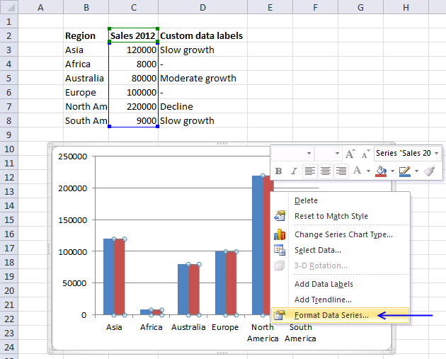
Custom data labels in a chart | Get Digital Help - Microsoft Excel resource
Post a Comment for "38 excel chart remove data labels"